Bayes Theorem and the Justice System November 22, 2009
Posted by Stephen Godfrey in Probability.Tags: Bayes theorem, general, justice, law, Maths, Probability
add a comment
I have been reading a previous issue of New Scientist and came across an article by Angela Saini which you can find here on how probability is used in the court room. Also if you goto the page you can take an online test to determine if the article is relevant for you next time you get stuck on jury duty.
It appears that to be a good jury member you need to have a good understanding of conditional and Bayesian Probability. So firstly what do I mean by conditional probability?
Let us consider two events 


because we already know that we have one dice being a 4 so the other dice also needs to be a 4 and that only happens one time in six.
Technical aside: To those probability nerds out there I know I should have labeled these dice, die 1 and die 2 to avoid any complications in finding 
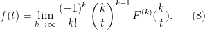
The actual definition of conditional probability is given as follows. If 

where we read 
The key point here is that the probability of an even occurring can change if we are given some extra information. Also note that if the two events are independent (i.e. are not related to each other) then 
Now what has this got to do with court cases? It has all to do with how some evidence will be presented in court, normally you should consider it as a conditional probability. We have all watched a some tv show that has involved some court case where an expert witness has said that “only 3% of the population has a AB blood type and so does the defendant” So what would we make of this in terms of probability?
Let 


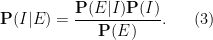
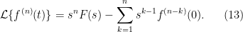
What we want to know is 
Let
Here you the jury would have a gut feel for what 


where 

Suppose that you are 80% certain that the defendant is innocent. So we have 

So once this evidence is given to you the defendants probable innocents plummets from 80% down to 22.4%. In this example you could still not convict using just this pice of evidence. What you can do is keep on adjusting
I will finish this post with four problems in understanding probabilities in court cases are (in no real order):
- 1) Prosecutor’s or Defendant’s Fallacy
- 2) Ultimate Issue Error Explicitly taking a small
- 3) Base-Rate Neglect
- 4) Dependent Evidence Fallacy This is related to the independence or dependence of events. In terms of court cases this would pop up in genetic effects. For instance we all know that certain physiological problems run in the family be it breast cancer or disease. If two events are independent from each other then the probability of both of these events happening can be found by multiplying both of the probabilities together.
However using the breast cancer example there is a 1/8 chance of a women having breast cancer during her life. So what is the probability of a mother and daughter both developing cancer during there lives. Well if mother has breast cancer then it is more likely that the daughter could develop breast cancer sometime during her life. I don’t know what that chance is so for sake of argument lets just say that it is twice as likely then the average person, that is a 1/4 chance. So we would find that there is a (1/8)(1/4)=1/32 chance that both mother and daughter will have cancer some time during there lives.
So this begs the question, if every one can be called up for jury duty should we be teaching more probability in schools so every one can understand trials that can include many confusing probabilities?
Integral Transforms and Partial Differential Equations October 21, 2009
Posted by Stephen Godfrey in Mathematics.Tags: Integral Transform, Maths
add a comment
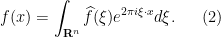
1. The Fourier and Laplace transform
This started off as a quick little post on solutions of PDE’s but my fingers took over and it has grown to become what it is now.
Every one that has done a maths degree would have seen both of these before, normally the Laplace transform while doing a course on ODE’s and the Fourier transform would come later once you know some measure theory. At least that was how it was for me.
If you have not head of them before or have not looked at them in the past few years and need a refresher please have a look at the above links. An interesting discussion of the Fourier transform is on Terry Tao’s blog here esp is you have seen LCA groups before.
There are many different definitions of the Fourier transform, all the same except for 
I will be taking this integral in the Lebesgue sense, however if you have never head of this integral before you can think of it as a normal integral. The difference between Lebesgue and Riemann integrals is that the former has a nicer theory under the hood.
The reason that you normally see the Fourier transform after doing some measure theory (Lebesgue Integral) is because of the particular spaces that 


The inverse Fourier transform is given by
Notice that the kernel or the transform is just the complex conjugate of the Fourier transform. (this is called). The trouble here is in what sense should we take this integral, what do we know about 

The Laplace transform is much more standard as it really only has one real formulation which we will take to be

First a note on notation, I am using the classical mathematical notation for these transforms. At some stage someone decided that the Fourier transform would be denoted by 
Secondly take note that I defined the Fourier transform over 


Thirdly there is a connection between the Laplace transform and the Fourier transform. Namely that if we assume that 


Indeed the Laplace and Fourier transform will share many similar properties. The reason that we don’t just study and use the Fourier transform is because the formulation of it is of great importance and is worthwhile looking at in this form.
The inversion of the Laplace transform is a little bit more problematic as there are several different approaches. I will not go into the details here, however I will provide a list of the most commonly used methods.
- 1) Partial Fraction decomposition This is normally the method first show to undergrad students. It is heavily dependent on having a large table of Laplace transforms.
- 2) Convolution Same as above but is useful for productions of transforms. The Laplace transform of a convolution of two functions can be shown to beIf we apply the inverse Laplace Transform to (5) we see that the product of two Laplace transforms can be inverted via a convolution,
- 3) Contour Integral Suppose that
exists for all
and is the Laplace transform of a piecewise continuous function
where
is greater then the real part of any of the singularities of
- 4) Post-Widder If the Laplace transform converges for some
, where
This formulation is more useful if you only want to know about the asymptotics of the solution.

2. Transform of Derivatives
Lets start by looking at the connection between the Fourier transform and derivatives and then Differential Equations.
I have already mentioned that I will be looking at the applying Integral transforms to solve Differential Equations. It will be convenient to introduce multi-index notation for derivatives. A multi-index 


and for polynomials 


The importance of the Fourier Transform for solving Differential Equations lies in the following result.
Theorem Let 

.
.
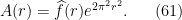
In (2) we also need the condition that 
Proof: The proof of these results on
The thing that you should take out of this is the following. Consider the Fourier transform as an operator 

An interesting question to ask is what is the Fourier transform of the operator

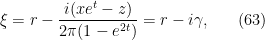
Observe that when the Fourier transform of 

The operator 
From this observation we see that using the Fourier transform to solve a differential equation involving a differential operator like
The Laplace transform has similar properties If 
3. Transform Solutions of PDE
We shall solve the classic PDE’s. The heat, wave and Laplace equations by Fourier transforms. We shall also solve the heat equation with different conditions imposed. The general method of solution will be the same. That is, we shall take the Fourier transform of the PDE and its initial and boundary conditions to reduce it to an ODE. We then solve this ODE for the transformed function. We invert this function to determine the solution to our PDE.
This is not just a method that is specific to the Fourier transform. This method also works for the Laplace transform and in general for many integral transforms. One condition on this is that the variable you take the integral transform its domain must match the range of integration of the integral transform. The type of boundary and initial conditions that are given can also play a role in which transform should be used. Once again I will devote a later post.
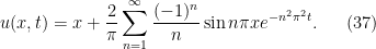
3.1. Example 1
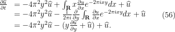
We consider the Cauchy problem for the heat equation on

with 

is the Laplacian on
![\displaystyle \begin{array}{ll} \int_{\mathbf{R}^n} \Delta u(x,t)e^{-2\pi ix\cdot \xi} dx &= \sum_{k=1}^{n} \int_{\mathbf{R}^n} \frac{\partial^2 u }{\partial x^2_k} e^{-2\pi ix\cdot \xi } d x\\ &=\left[\sum_{k=1}^{n} \frac{\partial u }{\partial x_k} e^{-2 \pi ix\cdot \xi }\right]_{|x|\rightarrow \infty} \\ &\qquad\qquad + \int_{\mathbf{R}^n} \sum_{k=1}^{n} 2\pi i\xi_k \frac{\partial u }{\partial x_k} e^{-2\pi ix\cdot \xi } d x\\ &=\sum_{k=1}^{n} 2\pi i\xi_k u(x,t) e^{-2 \pi ix\cdot \xi }|_{|x|\rightarrow \infty} \\ &\qquad+ \int_{\mathbf{R}^n} \sum_{k=1}^{n} (2\pi i\xi_k)^2 u(x,t) e^{-2\pi ix\cdot \xi } d x\\ &=-4 \pi^2 |\xi |^2 \widehat{u}. \end{array} \ \ \ \ \ (16)](https://s0.wp.com/latex.php?latex=%5Cdisplaystyle+%5Cbegin%7Barray%7D%7Bll%7D+%5Cint_%7B%5Cmathbf%7BR%7D%5En%7D+%5CDelta+u%28x%2Ct%29e%5E%7B-2%5Cpi+ix%5Ccdot+%5Cxi%7D+dx+%26%3D+%5Csum_%7Bk%3D1%7D%5E%7Bn%7D+%5Cint_%7B%5Cmathbf%7BR%7D%5En%7D+%5Cfrac%7B%5Cpartial%5E2+u+%7D%7B%5Cpartial+x%5E2_k%7D+e%5E%7B-2%5Cpi+ix%5Ccdot+%5Cxi+%7D+d+x%5C%5C+%26%3D%5Cleft%5B%5Csum_%7Bk%3D1%7D%5E%7Bn%7D+%5Cfrac%7B%5Cpartial+u+%7D%7B%5Cpartial+x_k%7D+e%5E%7B-2+%5Cpi+ix%5Ccdot+%5Cxi+%7D%5Cright%5D_%7B%7Cx%7C%5Crightarrow+%5Cinfty%7D+%5C%5C+%26%5Cqquad%5Cqquad+%2B+%5Cint_%7B%5Cmathbf%7BR%7D%5En%7D+%5Csum_%7Bk%3D1%7D%5E%7Bn%7D+2%5Cpi+i%5Cxi_k+%5Cfrac%7B%5Cpartial+u+%7D%7B%5Cpartial+x_k%7D+e%5E%7B-2%5Cpi+ix%5Ccdot+%5Cxi+%7D+d+x%5C%5C+%26%3D%5Csum_%7Bk%3D1%7D%5E%7Bn%7D+2%5Cpi+i%5Cxi_k+u%28x%2Ct%29+e%5E%7B-2+%5Cpi+ix%5Ccdot+%5Cxi+%7D%7C_%7B%7Cx%7C%5Crightarrow+%5Cinfty%7D+%5C%5C+%26%5Cqquad%2B+%5Cint_%7B%5Cmathbf%7BR%7D%5En%7D+%5Csum_%7Bk%3D1%7D%5E%7Bn%7D+%282%5Cpi+i%5Cxi_k%29%5E2+u%28x%2Ct%29+e%5E%7B-2%5Cpi+ix%5Ccdot+%5Cxi+%7D+d+x%5C%5C+%26%3D-4+%5Cpi%5E2+%7C%5Cxi+%7C%5E2+%5Cwidehat%7Bu%7D.+%5Cend%7Barray%7D+%5C+%5C+%5C+%5C+%5C+%2816%29&bg=ffffff&fg=000000&s=0&c=20201002)
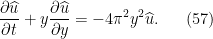
Therefore 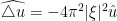
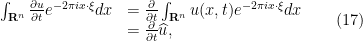
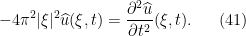
So if we take the Fourier transform of the Cauchy problem we get,

Taking the Fourier transform of the initial conditions gives,

We solve the ordinary differential equation above for 
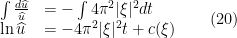
where 


Thus our solution is

Now taking the inverse Fourier transform to determine

Now as

we can rewrite 

where 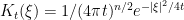

The function 


hence 
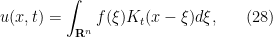
solves the heat equation with the given initial condition. Hence we have solved the Cauchy problem for the heat equation.
3.2. Example 2
Solve the heat equation

where 

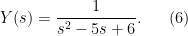
Taking the Laplace transform with respect to
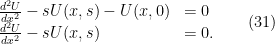
Solving this ODE we have

Now the Laplace transform of the conditions are
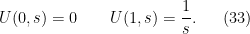
Using the boundary conditions we find that we have to solve the following system of equations

This system is easily solved as 


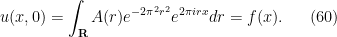
Now to find

Notice that all the singularities occur at 
If can be shown by the calculus of residues that the final solution is
3.3. Example 3
Let us start by considering the wave equation in 

We shall concern ourself with the wave equation on 

In fact when 
We also note that we can set 
We will solve the wave equation with Cauchy data. That is solve the problem
with the initial conditions

where 
Upon applying the standard technique for solving a partial differential equation by transform methods and treating 
Solving this ODE, we find the solution to be

where 


It is easy to see that

Therefore we find the solution of the ODE is
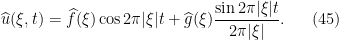
The solution of the wave equation is given by applying the inverse Fourier transform. As this has been a formal derivation let us be more precise. A solution of the Cauchy problem for the wave equation is
Proof: The proof is relatively simple. All you need to do is show that 

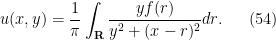
3.4. Example 4
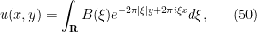
Solve the Laplace equation in the upper half plane

With the boundary condition 

Once again we find that 

To recover 


but from the initial condition,

so,

Now evaluating the inner integral,
![\displaystyle \begin{array}{ll} \int_{\mathbf{R}} e^{-2\pi |\xi |y+2\pi i\xi (x-r)} d \xi &= \int_{-\infty}^{0} e^{-2\pi |\xi |y+2\pi i\xi (x-r)}d \xi \\ &\qquad\qquad+ \int_{0}^{\infty} e^{-2\pi |\xi |y+2\pi i\xi (x-r)} d \xi \\ &=\int_{-\infty}^{0} e^{2\pi \xi (y+i(x-r) ) } d \xi \\ &\qquad\qquad+\int_{0}^{\infty} e^{-2\pi \xi (y+i(x-r) ) } d \xi \\ &=\left[\frac{e^{2\pi \xi (y+i(x-r) )}}{2\pi (y+i(x-r) )} \right]^{0}_{-\infty} +\left[\frac{-e^{-2\pi \xi (y+i(x-r) )}}{2\pi (y+i(x-r) )} \right]^{\infty}_{0}\\ &=\frac{1}{2\pi}\left(\frac{1}{y+i(x-r)}+\frac{1}{y-i(x-r)}\right)\\ &=\frac{1}{2\pi} \left(\frac{y+i(x-r)+y-i(x-r)}{y^2+(x-r)^2}\right)\\ &=\frac{y}{\pi (y^2+(x-r)^2)}. \end{array}\ \ \ \ \ (53)](https://s0.wp.com/latex.php?latex=%5Cdisplaystyle+%5Cbegin%7Barray%7D%7Bll%7D+%5Cint_%7B%5Cmathbf%7BR%7D%7D+e%5E%7B-2%5Cpi+%7C%5Cxi+%7Cy%2B2%5Cpi+i%5Cxi+%28x-r%29%7D+d+%5Cxi+%26%3D+%5Cint_%7B-%5Cinfty%7D%5E%7B0%7D+e%5E%7B-2%5Cpi+%7C%5Cxi+%7Cy%2B2%5Cpi+i%5Cxi+%28x-r%29%7Dd+%5Cxi+%5C%5C+%26%5Cqquad%5Cqquad%2B+%5Cint_%7B0%7D%5E%7B%5Cinfty%7D+e%5E%7B-2%5Cpi+%7C%5Cxi+%7Cy%2B2%5Cpi+i%5Cxi+%28x-r%29%7D+d+%5Cxi+%5C%5C+%26%3D%5Cint_%7B-%5Cinfty%7D%5E%7B0%7D+e%5E%7B2%5Cpi+%5Cxi+%28y%2Bi%28x-r%29+%29+%7D+d+%5Cxi+%5C%5C+%26%5Cqquad%5Cqquad%2B%5Cint_%7B0%7D%5E%7B%5Cinfty%7D+e%5E%7B-2%5Cpi+%5Cxi+%28y%2Bi%28x-r%29+%29+%7D+d+%5Cxi+%5C%5C+%26%3D%5Cleft%5B%5Cfrac%7Be%5E%7B2%5Cpi+%5Cxi+%28y%2Bi%28x-r%29+%29%7D%7D%7B2%5Cpi+%28y%2Bi%28x-r%29+%29%7D+%5Cright%5D%5E%7B0%7D_%7B-%5Cinfty%7D+%2B%5Cleft%5B%5Cfrac%7B-e%5E%7B-2%5Cpi+%5Cxi+%28y%2Bi%28x-r%29+%29%7D%7D%7B2%5Cpi+%28y%2Bi%28x-r%29+%29%7D+%5Cright%5D%5E%7B%5Cinfty%7D_%7B0%7D%5C%5C+%26%3D%5Cfrac%7B1%7D%7B2%5Cpi%7D%5Cleft%28%5Cfrac%7B1%7D%7By%2Bi%28x-r%29%7D%2B%5Cfrac%7B1%7D%7By-i%28x-r%29%7D%5Cright%29%5C%5C+%26%3D%5Cfrac%7B1%7D%7B2%5Cpi%7D+%5Cleft%28%5Cfrac%7By%2Bi%28x-r%29%2By-i%28x-r%29%7D%7By%5E2%2B%28x-r%29%5E2%7D%5Cright%29%5C%5C+%26%3D%5Cfrac%7By%7D%7B%5Cpi+%28y%5E2%2B%28x-r%29%5E2%29%7D.+%5Cend%7Barray%7D%5C+%5C+%5C+%5C+%5C+%2853%29&bg=ffffff&fg=000000&s=0&c=20201002)
Hence the solution to our problem is given by
3.5. Example 5
We already mentioned that to solve a non constant coefficient DE via the Fourier transform is not usually a useful approach. The same can be said for the Laplace transform. At the time we did mention that there are certain non constant coefficients PDE’s that can be solved by transforms methods. One example we mentioned was a Fokker-Plank equation.
In many applications such as in Finance a diffusion process is of importance. Often these diffusions are specified by a Fokker-Plank equation.
Let us solve the following Cauchy problem for a particular Fokker-Planck equation.

When we take the Fourier transform, this time we will not reduce the problem to that of solving an ODE. We will in fact end up with a first order partial differential equation.
Simplifying we have
We now have two options on how to proceed. We can solve this first order partial differential equation. However we can also take the Laplace transform in the
We shall first solve the first order PDE. By the method of characteristics we find the solution to be

where

where we made a substitution 

This implies that 
Now taking the inverse Fourier transform we have

After completing the square and setting
we find that
where we applied Cauchy’s Theorem in the last line. Evaluating the inner integral we find that

3.6. Example 6
Here we will look at solving a non constant coefficient that is in cylindrical co-ordinates.
where 


the boundary conditions turn into 


where 


To find out what 

After some calculations and the application of Cauchy’s integral formula at the zeros of 

where 


4. Final Remarks
From these examples there are a couple of important points to take away from them. First is that we need to match the domain of the variable we are going to transform to the range of the integration and what happens at the boundaries of your transform. Recall the Laplace transform required that you know initial values and the Fourier transform required decal at the ends of its domain.
The second point comes from the comparison of solving the constant coefficient (CC) and non CC PDE’s. When we were solving PDE’s with CC’s we were able to reduce the problem to solving a differential equation in one variable. In the non CC’s case we were able to reduce the order of the PDE by one.
This might lead you to think that we can blindly applying a Integral transform to a PDE to reduce the problem to something simpler. This is incorrect. Think of it this way our inversion formulas are also integral transforms. So if were were to take the inverse Fourier transform of

we would get Laplace’s equation. So here we have transformed an ODE to a second order PDE. Not much of a simplification.
What would be correct to think is that there is some connection between the kernel of the integral transform and the differential operator. Here the key is that 
So when you are solving a PDE using integral transforms you need to be mindful of both the domain (in particular the boundary). In a later post I will show how you can construct the “nicest” integral transform to solve a certain IVP or BVP. This makes use of Sturm-Liouville theory.
Introducing Integral Transforms October 14, 2009
Posted by Stephen Godfrey in Mathematics.Tags: Integral Transform, Maths
add a comment
As I spent the year studying I slowly found out that the current research in the field was rather different to what was doing in the classics, it appeared that I was born about 60-70 years too late. Most of the current research looks at new ways to invert Laplace transforms, deals with certain classes of distributions (also called Generalised functions), or plug a Hypergeometric function in the kernel. Not easy for work for an undergrad.
Now enough of this chit chat lets get into some maths!
The idea of using transformations in Mathematics is an old one. The idea is to change your problem into a simpler but equivalent problem, then change back to get the solution of the original problem. In this post I shall briefly explain why integrals transforms are useful when solving differential equations. The simplest answer is that one integral undoes one lot of differentiation, so if we integrate a ordinary differential equation we should only have an algebraic one.
The key point to remember is that we have mapped differentiation to something simpler like multiplication.
Integral transforms have been in wide use during the past two centuries as a tool to solve various problems in pure and applied mathematics. Many integral transforms were originally introduced to solve specific problems, but over the course of time have been found to be of use in the solution of other problems as well.
Let
 and let
  Let
Let

Then the mapping
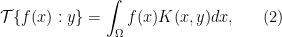
is an integral transform with domain 

There are several key questions that should be asked about any integral transform 
- What functions
- For every function
is there a unique function
?
- Given a function
, does there exist an operator that recovers
?
- What differential operator does this transform diagonalize?
For practical purposes the most important question that of if we can undo the transformation. With a bit of Functional Analysis we can answer this question for every integral transform. Since integration is linear it is easy to see that

The following lemma shows that if 
If a linear operator
from  into
into  is one-to-one, then there exists an operator
  , called the inverse of , such that
  and
and  , where
  and
and  are identity operators on and . The operator is also linear. Often is denoted by
  .
.It is important to note that although the linear operator
Many integral transforms share similar properties. What I intend to do is a quick survey of the well know integral transforms to look at the similarities as motivation to look for a more general framework of Integral transforms.
In an attempt to give a more general theory of integral transforms we shall attack this problem in three different ways, though self-adjoin DE’s, determining the relationship between the kernel in
Overall, as I mentioned above I will be interested in solving differential equations by integral transform methods. This is more out of personal interest as it is not the only place these transforms arise. The reason that integral transform methods are well suited to this problem is that many integral transforms convert certain differential operators into operators that act by multiplication.
As a simple example we consider the ordinary differential equation (ODE)

with the initial conditions 


which in turn can be solved for 

To find the solution to the differential equation we apply the inverse Laplace transform to
For Partial Differential Equations (PDE’s) we often do not reduce the equation to an algebraic problem. Often we reduce it to the problem of solving an ODE. Consider the inhomogeneous equation of telegraphy in the

By applying the Fourier transform in the

which is a much simpler problem to solve. In fact the solution to equation (8) can be shown to equal,

To find the solution to equation (7) we just apply the inverse Fourier transform to 
Although I will mainly be interested in solving problems like the previous two examples, I will also look at solving certain types of integral equations.
