Integral Transforms and Partial Differential Equations

Integral Transforms and Partial Differential Equations October 21, 2009

Posted by Stephen Godfrey in Mathematics.
Tags: Integral Transform, Maths
trackback

1. The Fourier and Laplace transform

This started off as a quick little post on solutions of PDE’s but my fingers took over and it has grown to become what it is now.

Every one that has done a maths degree would have seen both of these before, normally the Laplace transform while doing a course on ODE’s and the Fourier transform would come later once you know some measure theory. At least that was how it was for me.

If you have not head of them before or have not looked at them in the past few years and need a refresher please have a look at the above links. An interesting discussion of the Fourier transform is on Terry Tao’s blog here esp is you have seen LCA groups before.

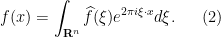
There are many different definitions of the Fourier transform, all the same except for ${2\pi}$ will appear in different places. In can be very annoying in the literature if someone uses a Fourier transform with out stating which one. I shall be using the following definition of the Fourier transform

I will be taking this integral in the Lebesgue sense, however if you have never head of this integral before you can think of it as a normal integral. The difference between Lebesgue and Riemann integrals is that the former has a nicer theory under the hood.

The reason that you normally see the Fourier transform after doing some measure theory (Lebesgue Integral) is because of the particular spaces that ${f}$ can live in so that the integral converges. Applying the triangle inequality it is east to see that the Fourier transform is defined if ${f\in L^1(\mathbf{R}^n)}$ This is a particular case of an Lp spaceWhen you get into more theory you can extend the underlying domain of the transform to Schawatrz functions or ${L^2(\mathbf{R}^n)}$ , for now I would recommend you have a look at Tao’s blog on the subject here.

The inverse Fourier transform is given by

$\displaystyle f(x)=\int_{\mathbf{R}^n} \widehat{f}(\xi) e^{2\pi i \xi\cdot x}d\xi. \ \ \ \ \ (2)$

Notice that the kernel or the transform is just the complex conjugate of the Fourier transform. (this is called). The trouble here is in what sense should we take this integral, what do we know about ${\widehat{f}(\xi)}$ ? Using the same argument as above we see that the inverse fourier transform is defined if ${\widehat{f}(\xi)\in L^1(\mathbf{R}^n)}$ , however this need not be the case. So what path should we take, we can either restrict ${f(x)}$ so that ${\widehat{f}(\xi)\in L^1(\mathbf{R}^n)}$ or we can extend the inversion formula to cover all possible situations. Both of these approaches have pro’s and con’s. Here we shall not concern ourselves with this technical problem and just assume that the maths gods are on our side! For this post we shall assume that this space is called ${A}$ . If you want to look at this in more detail please see….

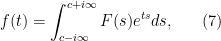
The Laplace transform is much more standard as it really only has one real formulation which we will take to be

$\displaystyle F(s)=\int_{0}^\infty f(t)e^{-st}dt. \ \ \ \ \ (3)$

First a note on notation, I am using the classical mathematical notation for these transforms. At some stage someone decided that the Fourier transform would be denoted by ${\widehat\cdot}$ and that the Laplace transform be denoted with a capital letter.

Secondly take note that I defined the Fourier transform over ${\mathbf{R}^n}$ and the Laplace transform over ${\mathbf{R}_+}$ . While we can take the Laplace transform over ${\mathbf{R}^n_+}$ by making the exponent of the Laplace transform to be an inner product of ${s}$ and ${t}$ , generally speaking we normally only take the Laplace transform in the time variable when we are solving a PDE so we don’t need the multidimensional version. I shall mention why the Laplace transform is well suited to these types of problems soon.

Thirdly there is a connection between the Laplace transform and the Fourier transform. Namely that if we assume that ${f(x)=0}$ for less than zero, then setting ${2\pi \xi=-si}$ gives

$\displaystyle \widehat{f}(\xi)=\widehat{f}(is/2\pi)=\int_0^\infty f(x)e^{-sx} dx=F(s). \ \ \ \ \ (4)$

Indeed the Laplace and Fourier transform will share many similar properties. The reason that we don’t just study and use the Fourier transform is because the formulation of it is of great importance and is worthwhile looking at in this form.

The inversion of the Laplace transform is a little bit more problematic as there are several different approaches. I will not go into the details here, however I will provide a list of the most commonly used methods.

1) Partial Fraction decomposition This is normally the method first show to undergrad students. It is heavily dependent on having a large table of Laplace transforms.
2) Convolution Same as above but is useful for productions of transforms. The Laplace transform of a convolution of two functions can be shown to beIf we apply the inverse Laplace Transform to (5) we see that the product of two Laplace transforms can be inverted via a convolution,
$\displaystyle f*g=\mathcal{L}^{-1}\{ F(s)G(s)\} \ \ \ \ \ (6)$
3) Contour Integral Suppose that ${F(s)}$ exists for all ${s>c}$ and is the Laplace transform of a piecewise continuous function ${f}$ . Then the Laplace transform can be inverted by the following contour integral
$\displaystyle f(t)=\int_{c-i\infty}^{c+i\infty} F(s)e^{ts}ds, \ \ \ \ \ (7)$

where ${c}$ is greater then the real part of any of the singularities of ${F(s)}$ .
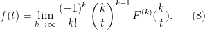
4) Post-Widder If the Laplace transform converges for some ${s>0}$ , where ${f}$ is a locally integrable function, then
$\displaystyle f(t)=\lim_{k\rightarrow \infty} \frac{(-1)^k}{k!} \left(\frac{k}{t}\right)^{k+1} F^{(k)}(\frac{k}{t}). \ \ \ \ \ (8)$

This formulation is more useful if you only want to know about the asymptotics of the solution.

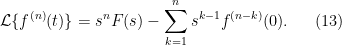
2. Transform of Derivatives

Lets start by looking at the connection between the Fourier transform and derivatives and then Differential Equations.

I have already mentioned that I will be looking at the applying Integral transforms to solve Differential Equations. It will be convenient to introduce multi-index notation for derivatives. A multi-index ${\alpha}$ is an ${n}$ -tuple of non-negative integers. If ${\alpha = (\alpha_1 ,\alpha_2 ,\dots , \alpha_n)}$ , define ${|\alpha |= \alpha_1 + \alpha_2 + \dots + \alpha_n }$ . We define ${D^\alpha}$ for any multi-index ${\alpha}$ by

$\displaystyle D^\alpha =\frac{\partial^{|\alpha |}}{\partial x_1^{\alpha_1}\partial x_2^{\alpha_2}\dots \partial x_n^{\alpha_n}}, \ \ \ \ \ (9)$

and for polynomials ${(\beta x)^\alpha}$ , where ${\beta\in \mathbf{R}}$ , we define it to be

$\displaystyle (\beta x)^\alpha =\beta^{|\alpha |} x_1^{\alpha_1} x_2^{\alpha_2} \dots x_n^{\alpha_n}. \ \ \ \ \ (10)$

The importance of the Fourier Transform for solving Differential Equations lies in the following result.

Theorem Let ${f}$ be an integrable function on ${\mathbf{R}}$ . Let ${\alpha}$ be a multi-index. Assume that ${f}$ is ${|\alpha|}$ times differentiable. Then

${\mathcal{F}\{D^\alpha f(x)\}=(2 \pi i \xi)^\alpha \widehat{f}(\xi)}$ .
${\mathcal{F}\{x^\alpha f(x)\}=\left(\dfrac{-1}{2 \pi i }\right)^{|\alpha|} D^\alpha \widehat{f}(\xi) }$ .

In (2) we also need the condition that ${x^\alpha f(x) \in L^1(\mathbf{R}^n)}$ .

Proof: The proof of these results on ${\mathbf{R}}$ can be found in many places. On ${\mathbf{R}^n}$ it is a simple case of induction. $\Box$

The thing that you should take out of this is the following. Consider the Fourier transform as an operator ${\widehat{f}:A\rightarrow \widehat{A}}$ , where ${A}$ is some space of functions that have Fourier transforms. It is interesting to note that differentiation on the space ${A}$ turns into multiplication by polynomials in the transform space ${\widehat{A}}$ . Furthermore multiplication by polynomials in ${A}$ turns into differentiation in ${\widehat{A}}$ .

An interesting question to ask is what is the Fourier transform of the operator

$\displaystyle L=\frac{d^n}{dx^n}+x^n? \ \ \ \ \ (11)$

Observe that when the Fourier transform of ${L}$ is taken, we get an operator that is of a similar form to ${L}$ back

$\displaystyle \mathcal{F} \{ L f(x) \}= (2\pi i \xi)^n \widehat{f}(\xi) +\left(\dfrac{-1}{2 \pi i }\right)^{n} \dfrac{ d ^n}{ d \xi^n} \widehat{f}(\xi). \ \ \ \ \ (12)$

The operator ${L}$ is almost a fixed point of the Fourier transform. When ${n=2}$ the operator ${L}$ is called the Harmonic oscillator.

From this observation we see that using the Fourier transform to solve a differential equation involving a differential operator like ${L}$ is unlikely to be a fruitful approach. In general the Fourier transform is not well suited to solving differential equations with non-constant coefficients. There are, however some problems of this type that can be solved by the Fourier transform. The example we will present later is a Fokker-Plank equation.

The Laplace transform has similar properties If ${F(s)}$ exists and ${f(t)}$ is ${n}$ times differentiable then,

$\displaystyle \mathcal{L} \{f^{(n)}(t)\}=s^n F(s)-\sum_{k=1}^n s^{k-1}f^{(n-k)}(0). \ \ \ \ \ (13)$

3. Transform Solutions of PDE

We shall solve the classic PDE’s. The heat, wave and Laplace equations by Fourier transforms. We shall also solve the heat equation with different conditions imposed. The general method of solution will be the same. That is, we shall take the Fourier transform of the PDE and its initial and boundary conditions to reduce it to an ODE. We then solve this ODE for the transformed function. We invert this function to determine the solution to our PDE.

This is not just a method that is specific to the Fourier transform. This method also works for the Laplace transform and in general for many integral transforms. One condition on this is that the variable you take the integral transform its domain must match the range of integration of the integral transform. The type of boundary and initial conditions that are given can also play a role in which transform should be used. Once again I will devote a later post.

3.1. Example 1

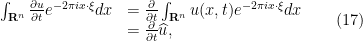
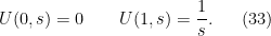
We consider the Cauchy problem for the heat equation on ${\mathbf{R}^n}$ . That is we solve

$\displaystyle \frac{\partial u}{\partial t}=\Delta u, \ \ \ \ \ (14)$

with ${u(x,0)=f(x),\quad f \in A}$ and where

$\displaystyle \Delta u(x,t)=\sum_{k=1}^{n} \frac{ \partial^2 u}{\partial x^2_k}, \ \ \ \ \ (15)$

is the Laplacian on ${\mathbf{R}^n}$ . Observe that,

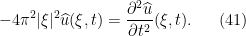
$\displaystyle \begin{array}{ll} \int_{\mathbf{R}^n} \Delta u(x,t)e^{-2\pi ix\cdot \xi} dx &= \sum_{k=1}^{n} \int_{\mathbf{R}^n} \frac{\partial^2 u }{\partial x^2_k} e^{-2\pi ix\cdot \xi } d x\\ &=\left[\sum_{k=1}^{n} \frac{\partial u }{\partial x_k} e^{-2 \pi ix\cdot \xi }\right]_{|x|\rightarrow \infty} \\ &\qquad\qquad + \int_{\mathbf{R}^n} \sum_{k=1}^{n} 2\pi i\xi_k \frac{\partial u }{\partial x_k} e^{-2\pi ix\cdot \xi } d x\\ &=\sum_{k=1}^{n} 2\pi i\xi_k u(x,t) e^{-2 \pi ix\cdot \xi }|_{|x|\rightarrow \infty} \\ &\qquad+ \int_{\mathbf{R}^n} \sum_{k=1}^{n} (2\pi i\xi_k)^2 u(x,t) e^{-2\pi ix\cdot \xi } d x\\ &=-4 \pi^2 |\xi |^2 \widehat{u}. \end{array} \ \ \ \ \ (16)$

Therefore ${\widehat{\triangle u}=-4 \pi^2 |\xi|^2 \hat{u}}$ . We now calculate the Fourier transform of the left hand side,

$\displaystyle \begin{array}{ll} \int_{\mathbf{R}^n} \frac{\partial u}{\partial t}e^{-2\pi i x\cdot \xi} d x &= \frac{\partial }{\partial t}\int_{\mathbf{R}^n} u(x,t)e^{-2\pi i x\cdot \xi}d x\\ &=\frac{\partial }{\partial t} \widehat{u}, \end{array}\ \ \ \ \ (17)$

So if we take the Fourier transform of the Cauchy problem we get,

$\displaystyle \frac{\partial \widehat{u}}{\partial t}=-4\pi^2 |\xi|^2 \widehat{u}. \ \ \ \ \ (18)$

Taking the Fourier transform of the initial conditions gives,

$\displaystyle \widehat{u}(y,0)=\int_{\mathbf{R}^n} f(x)e^{-2\pi i x\cdot \xi} d x=\widehat{f}(\xi) \ \ \ \ \ (19)$

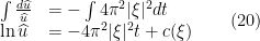
We solve the ordinary differential equation above for ${\widehat{u}(\xi,t)}$ . The ODE is separable, so that

$\displaystyle \begin{array}{ll} \int \frac{d\widehat{u}}{\widehat{u}}&= -\int 4\pi^2 |\xi|^2 d t\\ \ln{\widehat{u}}&= -4\pi^2 |\xi|^2 t+c(\xi) \end{array}\ \ \ \ \ (20)$

where ${c(\xi)}$ is an arbitrary factor of integration and is a function of ${\xi}$ . Hence ${\widehat{u}(\xi,t)=A(\xi)e^{-4\pi^2 |\xi|^2 t}}$ , where ${A(\xi)=e^{c(\xi)}}$ . But ${\widehat{u}(\xi,0)=\widehat{f}(\xi)}$ . Therefore,

$\displaystyle \widehat{u}(\xi,0)=\widehat{f}(\xi)=A(\xi)e^{0}. \ \ \ \ \ (21)$

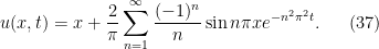
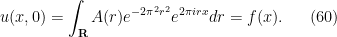
Thus our solution is

$\displaystyle \widehat{u}(\xi,t)=\widehat{f}(\xi)e^{-4\pi^2 |\xi|^2 t} \ \ \ \ \ (22)$

Now taking the inverse Fourier transform to determine ${u(x,t)}$

$\displaystyle \begin{array}{ll} u(x,t)&= \int_{\mathbf{R}^n} \widehat{f}(\xi)e^{-4\pi^2 |\xi|^2 t +2\pi ix\cdot \xi} d \xi\\ &=\int_{\mathbf{R}^n} \int_{\mathbf{R}^n} f(\eta )e^{-2\pi i\eta \cdot \xi} d\eta e^{-4\pi^2 |\xi|^2 t +2\pi ix\cdot \xi} d \xi \\ &=\int_{\mathbf{R}^n} \int_{\mathbf{R}^n} f(\eta ) e^{-4\pi^2 |\xi|^2 t +2\pi i(x-\eta )\cdot \xi} d \xi d \eta \\ &=\int_{\mathbf{R}^n} f(\eta ) \left(\int_{\mathbf{R}^n} e^{-4\pi^2 |\xi|^2 t +2\pi i(x-\eta )\cdot \xi} d\xi \right) d \eta . \end{array}\ \ \ \ \ (23)$

Now as

$\displaystyle \int_{\mathbf{R}^n} e^{-4\pi^2 |y|^2 t -2\pi i\omega \cdot y} d y=\frac{1}{(4\pi t)^{n/2}}e^{-|\omega|^2/4t}, \ \ \ \ \ (24)$

we can rewrite ${u(x,t)}$ as

$\displaystyle u(x,t)=\int_{\mathbf{R}^n} f(\xi ) K_t (x-\xi ) d \xi \ \ \ \ \ (25)$

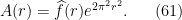
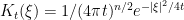
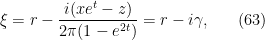
where ${K_t(\xi )=1/(4\pi t)^{n/2}e^{-|\xi|^2/4t}}$ and ${u(x,t)}$ could be rewritten as

$\displaystyle u(x,t)=f*K_t(x) \ \ \ \ \ (26)$

The function ${K_t (x)}$ is called the heat kernel on ${\mathbf{R}^n}$ . It is also called the Fundamental solution of the heat equation. It is easy to see that for all ${t>0}$ , ${K_t (x)}$ solves the heat equation. It is possible to show that the fundamental solution satisfies the initial condition

$\displaystyle \lim_{t\rightarrow 0}\int_{\mathbf{R}^n} f(\xi ) K_t(x-\xi ) d \xi =f(x), \ \ \ \ \ (27)$

hence ${\lim_{t\rightarrow 0} u(x,t)=f(x)}$ . So

$\displaystyle u(x,t)=\int_{\mathbf{R}^n} f(\xi ) K_t (x-\xi ) d \xi , \ \ \ \ \ (28)$

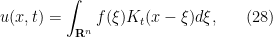
solves the heat equation with the given initial condition. Hence we have solved the Cauchy problem for the heat equation.

3.2. Example 2

Solve the heat equation

$\displaystyle \frac{\partial u}{\partial t}=\frac{\partial^2 u}{\partial x^2}, \ \ \ \ \ (29)$

where ${0<x<1}$ , ${t>0}$ and with the conditions that

$\displaystyle u(0,t)=0,\quad u(1,t)=1, \quad u(x,0)=0 \ \ \ \ \ (30)$

Taking the Laplace transform with respect to ${t}$ and denoting the Laplace transform with a capital we have

$\displaystyle \begin{array}{ll} \frac{d^2 U}{dx^2}-sU(x,s)-U(x,0)&=0\nonumber\\ \frac{d^2 U}{dx^2}-sU(x,s)&=0. \end{array}\ \ \ \ \ (31)$

Solving this ODE we have

$\displaystyle U(x,s)=c_1e^{\sqrt{s}x}+c_2e^{-\sqrt{s}x}. \ \ \ \ \ (32)$

Now the Laplace transform of the conditions are

$\displaystyle U(0,s)=0\qquad U(1,s)=\frac{1}{s}. \ \ \ \ \ (33)$

Using the boundary conditions we find that we have to solve the following system of equations

$\displaystyle \begin{array}{ll} 0&=c_1+c_2\\ \frac{1}{s}&=c_1e^{\sqrt{s}}+c_2e^{-\sqrt{s}} \end{array}\ \ \ \ \ (34)$

This system is easily solved as ${c_1=-c_2}$ so ${c_1=1/(s\sinh \sqrt{s})}$ . So our DE has the full solution of the form

$\displaystyle U(x,s)=\frac{\sinh x\sqrt{s}}{s \sinh \sqrt{s}}. \ \ \ \ \ (35)$

Now to find ${u(x,t)}$ we apply the complex inversion formula for the Laplace transform

$\displaystyle u(x,t)=\int_{c-i\infty}^{c+i\infty}\frac{\sinh x\sqrt{s}}{s \sinh \sqrt{s}}e^{st}ds. \ \ \ \ \ (36)$

Notice that all the singularities occur at ${s_n=-n^2\pi^2}$ . Each singularity is a simple pole.

If can be shown by the calculus of residues that the final solution is

$\displaystyle u(x,t)=x+\frac{2}{\pi} \sum_{n=1}^\infty \frac{(-1)^n}{n}\sin n\pi x e^{-n^2\pi^2 t}. \ \ \ \ \ (37)$

3.3. Example 3

Let us start by considering the wave equation in ${\mathbf{R}^n\times \mathbf{R}}$ . It is here that we start to run into some trouble about what the space ${A}$ should really be. If we were to take the space ${A=L^1(\mathbf{R}^n)}$ we would have a rather restrictive space as it does not include all of the solutions we can get from d’Alembert’s solution of the wave equation, where the solution does not even need to be continuous or integrable. However if we were to find solutions of this form using transform methods we would need to let ${A}$ be the space of tempered distributions, to do this would involve a great deal of preliminary work.

We shall concern ourself with the wave equation on ${n+1}$ -space

$\displaystyle \frac{\partial^2 u}{\partial x_1^2}+\cdots+\frac{\partial^2 u}{\partial x_n^2}=\frac{1}{c^2}\frac{\partial^2 u}{\partial t^2}. \ \ \ \ \ (38)$

In fact when ${n=3}$ the wave equation determines the behaviour of electromagnetic waves in a vacuum where ${c}$ will be the speed of light. It also models sound waves and many other forms of wave motion.

We also note that we can set ${c=1}$ with out any loss of generality, as we can rescale the equation.

We will solve the wave equation with Cauchy data. That is solve the problem

with the initial conditions

$\displaystyle u(x,0)=f(x)\qquad \frac{\partial u}{\partial t}(x,0)=g(x), \ \ \ \ \ (40)$

where ${f,g\in A}$ . Normally the ${t}$ variable to considered to be time. However we shall not restrict ${t}$ to be positive. In fact for our solution to the wave equation will make sense for any real value of ${t}$ . That is, the wave equation can be reversed in time.

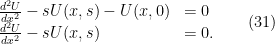
Upon applying the standard technique for solving a partial differential equation by transform methods and treating ${\xi}$ and ${x}$ a vectors we find that the Fourier transform of (39) is

$\displaystyle -4\pi^2|\xi|^2\widehat{u}(\xi,t)=\frac{\partial^2 \widehat{u}}{\partial t^2}(\xi,t). \ \ \ \ \ (41)$

Solving this ODE, we find the solution to be

$\displaystyle \widehat{u}(\xi,t)=A(\xi)\cos2\pi |\xi|t+B(\xi)\sin 2\pi|\xi|t, \ \ \ \ \ (42)$

where ${A(\xi)}$ and ${B(\xi)}$ are to be determined from the transformed initial conditions. These are

$\displaystyle \widehat{u}(\xi,0)=\widehat{f}(\xi)\quad\text{and}\quad\frac{\partial \widehat{u}}{\partial t}(\xi,0)=\widehat{g}(\xi). \ \ \ \ \ (43)$

It is easy to see that

$\displaystyle A(\xi)=\widehat{f}(\xi)\quad\text{and}\quad 2\pi|\xi|B(\xi)=\widehat{g}(\xi). \ \ \ \ \ (44)$

Therefore we find the solution of the ODE is

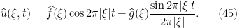
$\displaystyle \widehat{u}(\xi,t)=\widehat{f}(\xi)\cos 2\pi |\xi|t +\widehat{g}(\xi)\frac{\sin 2\pi |\xi|t}{2\pi |\xi|}. \ \ \ \ \ (45)$

The solution of the wave equation is given by applying the inverse Fourier transform. As this has been a formal derivation let us be more precise. A solution of the Cauchy problem for the wave equation is

Proof: The proof is relatively simple. All you need to do is show that ${u}$ satisfies the PDE and the extra conditions. $\Box$ The solution (46) is in fact a unique solution to the wave equation however we shall not prove this.

3.4. Example 4

Solve the Laplace equation in the upper half plane

$\displaystyle \frac{\partial^2 u }{\partial x^2 }+\frac{\partial^2 u }{\partial y^2 }=0,\quad x\in\mathbf{R}, \; y\geq 0 . \ \ \ \ \ (47)$

With the boundary condition ${u(x,0)=f(x)}$ . We will take the Fourier transform of the ${x}$ variable as it matched the domain of our transformation.

$\displaystyle \begin{array}{ll} \mathcal{F} \left\{\frac{\partial^2 u }{\partial x^2}+\frac{\partial^2 u }{\partial y^2 }\right\}&= 0\\ \frac{d^2 \widehat{u}}{d y^2}-4\pi^2 \xi^2 \widehat{u}&=0. \end{array}\ \ \ \ \ (48)$

Once again we find that ${\widehat{u}(\xi,0)=\widehat{f}(\xi)}$ . Now solving the ODE for ${\widehat{u} }$ ,

$\displaystyle \widehat{u}(\xi,y)=A(\xi )e^{2\pi |\xi |y}+B(\xi )e^{-2\pi |\xi |y}. \ \ \ \ \ (49)$

To recover ${u(x,y)}$ we have to take the inverse Fourier transform. But the inverse Fourier transform of ${e^{2\pi|\xi|y}}$ does not exist. So we have to set ${A(\xi)=0}$ . Hence,

$\displaystyle u(x,y)=\int_{\mathbf{R}}B(\xi) e^{-2\pi |\xi |y+2\pi i \xi x}d \xi, \ \ \ \ \ (50)$

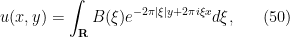
but from the initial condition,

$\displaystyle \widehat{u}(\xi ,0)=\widehat{f}(\xi )=B(\xi )e^0 =B(\xi ) , \ \ \ \ \ (51)$

so,

$\displaystyle \begin{array}{ll} u(x,y)&= \int_{\mathbf{R}} \widehat{f}(\xi )e^{-2\pi |\xi |y+2\pi i\xi x} d \xi\\ &=\int_{\mathbf{R}} \int_{\mathbf{R}} f(r)e^{-2\pi i \xi r}dr e^{-2\pi |\xi |y+2\pi i\xi x} d \xi\\ &=\int_{\mathbf{R}} f(r) \left(\int_{\mathbf{R}} e^{-2\pi |\xi |y+2\pi i\xi (x-r)}d\xi \right) d r. \end{array}\ \ \ \ \ (52)$

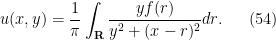
Now evaluating the inner integral,

$\displaystyle \begin{array}{ll} \int_{\mathbf{R}} e^{-2\pi |\xi |y+2\pi i\xi (x-r)} d \xi &= \int_{-\infty}^{0} e^{-2\pi |\xi |y+2\pi i\xi (x-r)}d \xi \\ &\qquad\qquad+ \int_{0}^{\infty} e^{-2\pi |\xi |y+2\pi i\xi (x-r)} d \xi \\ &=\int_{-\infty}^{0} e^{2\pi \xi (y+i(x-r) ) } d \xi \\ &\qquad\qquad+\int_{0}^{\infty} e^{-2\pi \xi (y+i(x-r) ) } d \xi \\ &=\left[\frac{e^{2\pi \xi (y+i(x-r) )}}{2\pi (y+i(x-r) )} \right]^{0}_{-\infty} +\left[\frac{-e^{-2\pi \xi (y+i(x-r) )}}{2\pi (y+i(x-r) )} \right]^{\infty}_{0}\\ &=\frac{1}{2\pi}\left(\frac{1}{y+i(x-r)}+\frac{1}{y-i(x-r)}\right)\\ &=\frac{1}{2\pi} \left(\frac{y+i(x-r)+y-i(x-r)}{y^2+(x-r)^2}\right)\\ &=\frac{y}{\pi (y^2+(x-r)^2)}. \end{array}\ \ \ \ \ (53)$

Hence the solution to our problem is given by

$\displaystyle u(x,y)=\frac{1}{\pi}\int_{\mathbf{R}} \frac{y f(r)}{y^2 +(x-r)^2} dr. \ \ \ \ \ (54)$

3.5. Example 5

We already mentioned that to solve a non constant coefficient DE via the Fourier transform is not usually a useful approach. The same can be said for the Laplace transform. At the time we did mention that there are certain non constant coefficients PDE’s that can be solved by transforms methods. One example we mentioned was a Fokker-Plank equation.

In many applications such as in Finance a diffusion process is of importance. Often these diffusions are specified by a Fokker-Plank equation.

Let us solve the following Cauchy problem for a particular Fokker-Planck equation.

$\displaystyle \frac{\partial u}{\partial t}=\frac{\partial^2 u}{\partial x^2}+x\frac{\partial u}{\partial x}+u,\qquad u(x,0)=f(x). \ \ \ \ \ (55)$

When we take the Fourier transform, this time we will not reduce the problem to that of solving an ODE. We will in fact end up with a first order partial differential equation.

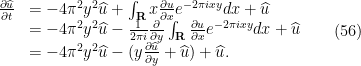
$\displaystyle \begin{array}{ll} \frac{\partial \widehat{u}}{\partial t}&=-4\pi^2y^2\widehat{u}+\int_{\mathbf{R}} x\frac{\partial u}{\partial x}e^{-2\pi ixy}dx+\widehat{u}\\ &=-4\pi^2y^2\widehat{u}-\frac{1}{2\pi i} \frac{\partial}{\partial y}\int_{\mathbf{R}} \frac{\partial u}{\partial x}e^{-2\pi ixy}dx+\widehat{u}\\ &=-4\pi^2y^2\widehat{u}-(y\frac{\partial \widehat{u}}{\partial y}+\widehat{u})+\widehat{u}. \end{array}\ \ \ \ \ (56)$

Simplifying we have

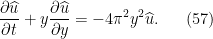
$\displaystyle \frac{\partial \widehat{u}}{\partial t}+y\frac{\partial \widehat{u}}{\partial y}=-4\pi^2y^2\widehat{u}. \ \ \ \ \ (57)$

We now have two options on how to proceed. We can solve this first order partial differential equation. However we can also take the Laplace transform in the ${t}$ variable and reduce the problem to that of solving an ODE.

We shall first solve the first order PDE. By the method of characteristics we find the solution to be

$\displaystyle \widehat{u}(y,t)=A(y)e^{-t}e^{-2\pi^2y^2}, \ \ \ \ \ (58)$

where ${A}$ is unknown. To recover ${u}$ we apply the inverse Fourier transform. So

$\displaystyle \begin{array}{ll} u(x,t)&=\int_{\mathbf{R}} A(y)e^{-t}e^{-2\pi^2y^2}e^{2\pi i yx}dy\\ &=\int_{\mathbf{R}} A(r) e^{-2\pi^2r^2e^{2t}}e^{2\pi i rxe^{t}}e^{t}dr, \end{array}\ \ \ \ \ (59)$

where we made a substitution ${r=ye^{-t}}$ . Now ${u(x,0)=f(x)}$ , so ${\widehat{u}(y,0)=\widehat{f}(y)}$ . So we have that

$\displaystyle u(x,0)=\int_{\mathbf{R}} A(r)e^{-2\pi^2r^2}e^{2\pi i rx}dr=f(x). \ \ \ \ \ (60)$

This implies that ${A(r)e^{-2\pi^2r^2}=\widehat{f}(r)}$ . Thus

$\displaystyle A(r)=\widehat{f}(r)e^{2\pi^2r^2}. \ \ \ \ \ (61)$

Now taking the inverse Fourier transform we have

$\displaystyle \begin{array}{ll} u(x,t)&=\int_{\mathbf{R}} \widehat{f}(r)e^{2\pi^2r^2}e^{-2\pi^2r^2e^{2t}}e^{2\pi i rxe^{t}}e^{t}dr\\ &=\int_{\mathbf{R}} f(z) \left( \int_{\mathbf{R}} e^{-2\pi^2 r^2(1-e^{2t})}e^{2\pi i r(xe^{t}-z)}e^t dr \right)dz. \end{array}\ \ \ \ \ (62)$

After completing the square and setting

$\displaystyle \xi=r-\frac{i(xe^{t}-z)}{2\pi(1-e^{2t})}=r-i\gamma, \ \ \ \ \ (63)$

we find that

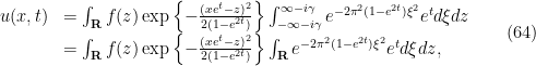
$\displaystyle \begin{array}{ll} u(x,t)&=\int_{\mathbf{R}} f(z) \exp \left\{ -\frac{(xe^t-z)^2}{2(1-e^{2t})} \right\}\int_{-\infty -i\gamma}^{\infty -i\gamma} e^{-2\pi^2(1-e^{2t})\xi^2} e^t d\xi dz\\ &= \int_{\mathbf{R}} f(z)\exp \left\{ -\frac{(xe^t-z)^2}{2(1-e^{2t})}\right\} \int_{\mathbf{R}} e^{-2\pi^2(1-e^{2t})\xi^2} e^t d\xi dz, \end{array}\ \ \ \ \ (64)$

where we applied Cauchy’s Theorem in the last line. Evaluating the inner integral we find that

$\displaystyle u(x,t)=\int_{\mathbf{R}} f(z)\frac{e^t}{\sqrt{2\pi (1-e^{2\pi}})} \exp \left\{ -\frac{(xe^t-z)^2}{2(1-e^{2t})} \right\} dz. \ \ \ \ \ (65)$

3.6. Example 6

Here we will look at solving a non constant coefficient that is in cylindrical co-ordinates.

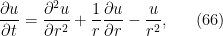
$\displaystyle \frac{\partial u}{\partial t}=\frac{\partial^2 u}{\partial r^2}+\frac{1}{r}\frac{\partial u}{\partial r}-\frac{u}{r^2}, \ \ \ \ \ (66)$

where ${0<r<1}$ and ${t>0}$ such that ${u(0,t)=0}$ and ${u(1,t)=1}$ with initial condition ${u(r,0)}$ . The Laplace transform of this PDE is

$\displaystyle r^2U(r,s)+rU_r(r,s)-(r^2s+1)U(r,s)=0, \ \ \ \ \ (67)$

the boundary conditions turn into ${U(0,s)=0}$ and ${U(1,s)=1/s}$ . The general solution of the ODE is

$\displaystyle U(r,s)=A I_1(r\sqrt{s})+B K_1(r\sqrt{s}), \ \ \ \ \ (68)$

where ${I_1(\cdot)}$ and ${K_1(\cdot)}$ are the first order modified Bessel functions of the second kind. Now as ${K_1(\cdot)}$ is unbounded at the origin we set ${B=0}$ . Applying the Boundary conditions gives

$\displaystyle U(r,s)=\frac{I_1(r\sqrt{s})}{s I_1(\sqrt{s})}. \ \ \ \ \ (69)$

To find out what ${u(r,t)}$ is we need to compute the integral

$\displaystyle \frac{1}{2\pi i} \oint_C \frac{I_1(r\sqrt{s})}{s I_1(\sqrt{s})} e^{ts}ds. \ \ \ \ \ (70)$

After some calculations and the application of Cauchy’s integral formula at the zeros of ${I_1(\sqrt{s})}$ we have

$\displaystyle u(r,t)=r+2\sum_{n=1}^\infty \frac{J_1(\alpha_n r)}{\alpha_n J_0(\alpha_n)}e^{-\alpha_n^2 t}, \ \ \ \ \ (71)$

where ${\alpha_n}$ are the zeros of the Bessel function ${J_1(\cdot)}$ for ${n=1,2,\dots}$ .

4. Final Remarks

From these examples there are a couple of important points to take away from them. First is that we need to match the domain of the variable we are going to transform to the range of the integration and what happens at the boundaries of your transform. Recall the Laplace transform required that you know initial values and the Fourier transform required decal at the ends of its domain.

The second point comes from the comparison of solving the constant coefficient (CC) and non CC PDE’s. When we were solving PDE’s with CC’s we were able to reduce the problem to solving a differential equation in one variable. In the non CC’s case we were able to reduce the order of the PDE by one.

This might lead you to think that we can blindly applying a Integral transform to a PDE to reduce the problem to something simpler. This is incorrect. Think of it this way our inversion formulas are also integral transforms. So if were were to take the inverse Fourier transform of

$\displaystyle \frac{d^2 \widehat{u}}{d y^2}-4\pi^2 \xi^2 \widehat{u}=0, \ \ \ \ \ (72)$

we would get Laplace’s equation. So here we have transformed an ODE to a second order PDE. Not much of a simplification.

What would be correct to think is that there is some connection between the kernel of the integral transform and the differential operator. Here the key is that ${e^{\omega x}}$ is generally a solution of a second order differential equation with constant coefficients.

So when you are solving a PDE using integral transforms you need to be mindful of both the domain (in particular the boundary). In a later post I will show how you can construct the “nicest” integral transform to solve a certain IVP or BVP. This makes use of Sturm-Liouville theory.

Comments»

No comments yet — be the first.

Stevethemathsman's Blog