Introducing Integral Transforms October 14, 2009
Posted by Stephen Godfrey in Mathematics.Tags: Integral Transform, Maths
trackback
As I spent the year studying I slowly found out that the current research in the field was rather different to what was doing in the classics, it appeared that I was born about 60-70 years too late. Most of the current research looks at new ways to invert Laplace transforms, deals with certain classes of distributions (also called Generalised functions), or plug a Hypergeometric function in the kernel. Not easy for work for an undergrad.
Now enough of this chit chat lets get into some maths!
The idea of using transformations in Mathematics is an old one. The idea is to change your problem into a simpler but equivalent problem, then change back to get the solution of the original problem. In this post I shall briefly explain why integrals transforms are useful when solving differential equations. The simplest answer is that one integral undoes one lot of differentiation, so if we integrate a ordinary differential equation we should only have an algebraic one.
The key point to remember is that we have mapped differentiation to something simpler like multiplication.
Integral transforms have been in wide use during the past two centuries as a tool to solve various problems in pure and applied mathematics. Many integral transforms were originally introduced to solve specific problems, but over the course of time have been found to be of use in the solution of other problems as well.
Let
 and let
 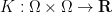 Let
Let

Then the mapping
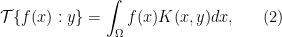
is an integral transform with domain 


There are several key questions that should be asked about any integral transform 
- What functions
are in
- For every function
is there a unique function
?
- Given a function
, does there exist an operator that recovers
?
- What differential operator does this transform diagonalize?
For practical purposes the most important question that of if we can undo the transformation. With a bit of Functional Analysis we can answer this question for every integral transform. Since integration is linear it is easy to see that

The following lemma shows that if 
If a linear operator
 from
from  into
into  is one-to-one, then there exists an operator
  , called the inverse of , such that
  and
and  , where
  and
and  are identity operators on and . The operator is also linear. Often is denoted by
  .
.It is important to note that although the linear operator
Many integral transforms share similar properties. What I intend to do is a quick survey of the well know integral transforms to look at the similarities as motivation to look for a more general framework of Integral transforms.
In an attempt to give a more general theory of integral transforms we shall attack this problem in three different ways, though self-adjoin DE’s, determining the relationship between the kernel in
Overall, as I mentioned above I will be interested in solving differential equations by integral transform methods. This is more out of personal interest as it is not the only place these transforms arise. The reason that integral transform methods are well suited to this problem is that many integral transforms convert certain differential operators into operators that act by multiplication.
As a simple example we consider the ordinary differential equation (ODE)

with the initial conditions 


which in turn can be solved for 

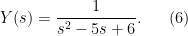
To find the solution to the differential equation we apply the inverse Laplace transform to
For Partial Differential Equations (PDE’s) we often do not reduce the equation to an algebraic problem. Often we reduce it to the problem of solving an ODE. Consider the inhomogeneous equation of telegraphy in the 

By applying the Fourier transform in the

which is a much simpler problem to solve. In fact the solution to equation (8) can be shown to equal,

To find the solution to equation (7) we just apply the inverse Fourier transform to 
Although I will mainly be interested in solving problems like the previous two examples, I will also look at solving certain types of integral equations.

Comments»
No comments yet — be the first.